Article Text

Statistics from Altmetric.com
Confounding should always be addressed in studies concerned with causality. When present, it results in a biased estimate of the effect of exposure on disease. The bias can be negative—resulting in underestimation of the exposure effect—or positive, and can even reverse the apparent direction of effect. It is a concern no matter what the design of the study or what statistic is used to measure the effect of exposure.
The potential for confounding can be reduced by good study design, but in non-randomised studies this is unlikely to resolve the problem fully. Hence statistical adjustment methods, to reduce the bias caused by measured confounders, are also frequently considered. Such adjustment presupposes that one knows which factors are confounders. However, recent literature on methods for identifying confounders suggest that these are not always obvious. Indeed, in pursuit of guidelines, authors have had to reexamine the meanings of confounding and confounders with some ambiguity and conflict emerging. This literature is reviewed and a recent modification to the traditional definition of a confounder, which emphasises causal rather than statistical relationships, is described and illustrated. Some well known problems in occupational epidemiology, arising from health related selection, are considered in the light of recent ideas.
Control of confounding through study design is not addressed, nor is the article concerned with details of statistical methods for adjustment. An overview of design and analysis in relation to confounding by age may be useful additional reading.1 It is assumed that the reader has at least a basic knowledge of epidemiological methods. Unless otherwise stated, definitions and comments apply to all causal study designs including case–control studies.
DEFINITIONS
Example
Consider a study of the relationship between exposure to silica dust and lung cancer where the rate of lung cancer in exposed workers is twice that in unexposed subjects, giving a rate ratio (RR) of two. The RR is a measure of the size of the effect of silica exposure on risk; here it suggests that exposure to silica dust is a cause of lung cancer. However, there might be other explanations for the increased rate among the exposed: if 50% of exposed workers were lifelong tobacco smokers compared to 30% of unexposed subjects, then this difference might explain some of the increase. This would then suggest that the true effect of silica exposure is less than two and that the result, RR = 2, is positively biased; smoking might be labelled a confounder of the relationship between silica and lung cancer. A statistical adjustment method could be used to try to estimate the true, unconfounded effect of exposure.
The traditional criteria for identifying confounders are the first three conditions C1–C3 in box 1. In the previous example, tobacco smoking fulfils all the criteria; it is a cause of lung cancer and it is correlated (associated) with silica exposure in this study population. There is unlikely to be a causal pathway (C3) linking silica exposure to smoking and then to lung cancer, since silica exposure is unlikely to be a cause of smoking. Thus smoking probably is a confounder in this study but, as discussed later, this checklist for identifying confounders is not foolproof and a change has been recommended. First, it is useful to consider the meaning of confounding, a concept which can be defined independently of the definition of a confounder.
Causal effects and confounding
Pearl2 notes that “confounding is a causal concept”; it is only of interest because it is an impediment to learning about genuine causal effects. To recognise confounding, one ought perhaps firstly to understand what is meant by causal effect. In fact this frequently invoked concept is difficult to pin down, as evidenced by the variety of definitions proposed by philosophers and scientists over the centuries. One of these, attributed to Neyman in 1923, and also to Rubin in 1974, has been the focus of recent epidemiological interest3 since it leads naturally to a definition of confounding.
Suppose we are interested in whether an exposure over a period of time, P, causes pain in the head at a later time point. The causal effect of the exposure on a particular individual is defined as the difference between the level of pain the individual would feel if she was exposed during P and the pain level if she was not exposed during P. Likewise, in a group of subjects, the average causal effect is defined as the difference between average pain levels. For disease outcomes, the (average) causal effect of exposure during a period of work, P1, on disease incidence in a group during a period, P2, is the difference between:
A: the incidence during P2 if they were exposed during P1, and
B: the incidence during P2 if they were not exposed during P1.
Box 1: Confounders—old and new necessary conditions
The factor must:
-
C1 be a cause of the disease, or a surrogate measure of a cause, in unexposed people; factors satisfying this condition are called risk factors and
-
C2 be correlated, positively or negatively, with exposure in the study population. If the study population is classified into exposed and unexposed groups, this means that the factor has a different distribution (prevalence) in the two groups and
-
C3not be an intermediate step in the causal pathway between the exposure and the disease
New stricter condition, now replacing C3:
-
C3anot be affected by the exposure
In these definitions, a zero difference would mean that the exposure had no (zero) causal effect.
These definitions are clear cut but the problem of finding empirical data to meet their requirements is not. To measure the causal effect of exposure on disease occurrence requires a contrast between the experience of a group exposed during P1 with the experience of these same subjects had they been unexposed during P1. This is impossible, since subjects cannot both be exposed and unexposed at the same time. It follows that perfect evidence of causal effects is unattainable. Nevertheless, in practice, we search for the best available—that is, observable—evidence. Hence, given the disease experience, A, of a group of exposed subjects, we look for some observable experience with which to compare it, as a substitute for the unobservable B—for example, the disease experience of a different set of subjects: the “unexposed group”. If the incidence in this unexposed group is equal to the hypothetical incidence of “the exposed group, had they been unexposed”, then the substitution is perfect. But if it is not, the comparison will give a false picture of the causal effect of exposure and it is said to be confounded.3 The key issue in confounding is therefore the comparability of exposed and unexposed subjects, if both had been unexposed (box 2). The second definition4,5 in box 2 spells out the consequence of confounding—that is, bias.
Confounders
In practice, we address confounding through searching for and controlling confounders: these are the disease risk factors which are jointly responsible for the lack of comparability of exposed and unexposed. Most textbooks to date have defined a confounder in terms of C1–C3; however these conditions are necessary, but not sufficient, to cause confounding. By “necessary, but not sufficient” we mean that:
-
all confounders must satisfy these conditions, but
-
some factors which satisfy all three conditions may not cause confounding.
Box 2: Confounding as non-comparability
Confounding is:
-
a lack of comparability between exposed and unexposed groups arising because, had the exposed actually been unexposed, their disease risk would have been different from that in the actual unexposed group
-
a bias in the estimation of the effect of exposure on disease, due to inherent differences in risk between exposed and unexposed groups
One reason why factors might not produce confounding, though satisfying C1–C3, is that their potential confounding effects might cancel out.6 Consider the example of silica dust and lung cancer discussed earlier; suppose that, in addition to the greater prevalence of smoking in the exposed group, these subjects are also much younger than unexposed subjects. Both age and smoking would then satisfy C1–C3; however, because their potential biasing effects are in opposite directions, it is possible that these cancel each other out. If so, and if there are no other differences between exposed and unexposed, there would be no confounding. Situations where potential biases cancel out completely are probably rare in practice and so ought not to be stressed. Nevertheless a related point, that biases in opposite directions may partially cancel, and that the overall degree of confounding is determined by the net effect of these potential biases, is relevant to practice.
A more important criticism of the definition C1–C3 is that it does not fully distinguish the reasons for the association between the suspected confounder and exposure implied by C2.7 There are several reasons why a suspected confounder, S, and exposure, E, might be associated in a study: E may cause S, S may cause E, both may have a common cause, or the reason may be entirely non-causal—for example, selection bias. A modification of the traditional confounder definition, now accepted in the latest epidemiological textbooks, states that if S is caused by E, then S should not be regarded as a confounder. This new condition—see C3a in box 1—replaces C3 which is just a special case of it, so that the new joint criteria for a confounder are C1, C2, and C3a.8
The introduction of C3a reflects a growing understanding that reliance on purely statistical rules, as opposed to rules defined by causal relationships, can lead to some factors being wrongly labelled as confounders; furthermore, standard statistical adjustments for such factors could produce bias rather than remove it.2,9 Figure 1 uses “causal graphs” to illustrate how use of C3a can avoid these mistakes. In causal graphs, an arrow from one variable to another variable indicates that the former is a cause of the latter; likewise, a chain of unidirectional arrows implies a causal relationship.
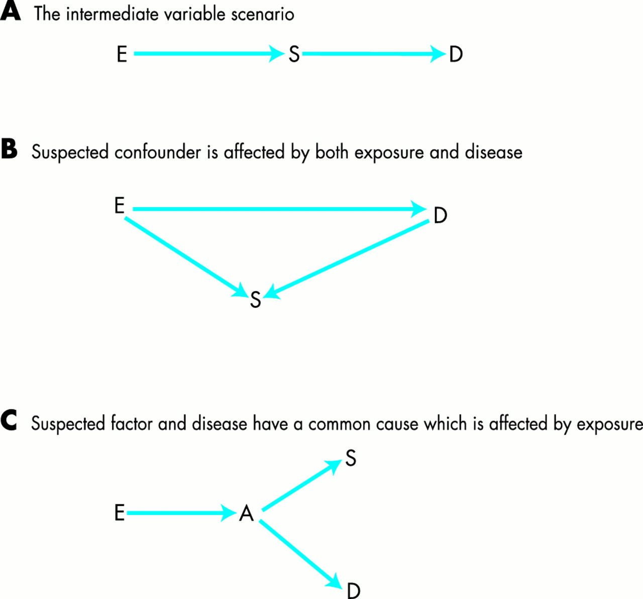
Causal diagrams where suspected factor, S, is affected by exposure and therefore not a confounder. E and D are respectively the exposure and disease whose relationship is under study; S is the (falsely) suspected confounder; A is a common cause of S and D.
In fig 1A the suspected confounder S lies on the causal pathway between E and disease, D; S is part of the mechanism whereby E causes D. Application of criterion C3a—or C3—tells us that S is not a confounder and we should not “adjust” for it. Suppose that shift work (E) causes cardiovascular disease (D) by impairing glucose tolerance and consider a study of the E–D association in which glucose tolerance was measured five years after shift work began (S). If fig 1A correctly portrays these relationships, then adjustment for S would be wrong. Note that E→S implies only that shift work is a cause of glucose intolerance, not the only cause. As a counter example, consider the same study but with glucose tolerance measured before workers took up shift work: now fig 1A is inappropriate since the relationship E→S cannot be true. In this case, S might even be treated as a confounder—for example, if it was found that those who became shift workers had lower glucose tolerances before going into shift work than day workers. Note how causal graphs enable these contrasting situations to be easily distinguished by forcing us to think about the causal directions underlying associations.
A famous example of the scenario in fig 1B is the relationship between oestrogen use, E and endometrial cancer, D, where the question arises as to whether uterine bleeding, S, is a confounder. Since uterine bleeding is not a cause of endometrial cancer, C1 alone would lead to the (correct) conclusion that it is not. However, in one study of this relationship, it was thought that endometrial cancer might be diagnosed more readily in women taking oestrogen who bled, and that this problem could be solved by “controlling” for uterine bleeding. Control was through study design rather than analysis; as later became clear, it led to a greatly reduced, biased estimate of the true relationship.9 Criterion C3a leads straightforwardly to the correct conclusion that it should not be treated as a confounder. The relationships in this figure might also be found when E refers to an occupational exposure—for example, S might be chronic cough and D lung cancer; the same conclusions would apply.
As an example fitting fig 1C, Weinberg7 considered a study of the effect of exposure, E, on the risk of spontaneous abortion in current pregnancy, D, where the question arises as to whether a history of spontaneous abortion in a previous pregnancy, S, should be treated as a confounder. The assumptions in fig 1C are that both spontaneous abortion in current and previous pregnancies are caused by the same underlying abnormality, A—for example, A might be poor response of the endometrium to endogenous oestrogens. Exposure is a cause of A. The pathway E→A→S implies that exposure is also a cause of S, previous spontaneous abortion; therefore according to C3a, S should not be treated as a confounder. For further discussion of this example, the reader is referred to the original paper and the publications and correspondence provoked by it. Note that in all the examples here, the conclusions about confounders relate to the causal assumptions illustrated: other causal assumptions might lead to different conclusions.
The new joint criteria—C1, C2, and C3a—should be regarded as the currently best available, simple guide to confounder identification, while recognising that it is still not foolproof. In fact a watertight method for identification of confounders exists but elaboration of this important work by Pearl2 is beyond the scope of the present article. In brief, it requires construction of a causal diagram which summarises knowledge/assumptions about all of the causal relationships between exposure, disease, and all suspected confounders. The set of true confounders are then identified from the graph by applying a graphical algorithm. Application of the method to epidemiological research, and its relationship to the criteria C1–C3a, has been discussed elsewhere.9 It is likely that the two methods will agree in many cases but situations where there are multiple potential confounders, many causally related to each other, may require the additional insight offered by Pearl’s algorithm.
Empirical evidence of confounding: internal versus external evidence
The last section stressed the need to address causal relationships when searching for confounders. But this very aspect can lead to difficulties in the practice of identifying confounders since causality cannot be established from data alone. In grappling with this problem, it is useful to distinguish between two types of evidence: internal, statistical evidence from the “data at hand”, and external evidence such as prior research and prior beliefs. The relative importance of these two sources, especially if they appear to conflict, needs to be established for each of the criteria C1–C3a.
Suppose that data on disease, D, and a potential confounder, S, are available and consider the evidence that S is a cause of D. If D were lung cancer and S tobacco smoking then, regardless of what the data at hand showed, one would regard tobacco smoking as a risk factor for lung cancer because of strong external evidence. If instead S were “match carrying”, it would be rejected as a risk factor, despite what the data might suggest, because of a strong belief that a causal relationship is implausible.6,8 These examples illustrate that strong external evidence about C1 can override internal evidence: what matters is the true causal relationship between S and disease, not how that relationship appears in the data at hand.6
Sometimes there is little or no prior evidence about the causal effect of S so that there is more reliance on internal data. It is important to recognise that data based evidence, about whether S is a risk factor, may itself suffer from confounding. For example, a crude analysis might show an association between alcohol consumption, S, and lung cancer when in reality there is no causal relationship: the apparent association could be due to confounding by smoking. To see whether alcohol is truly a risk factor, one would need to adjust for smoking. In general, the decision as to whether S is a risk factor for D should be based on suitably adjusted associations.
Both C2 and C3a refers to the relationship between E and S: C2 seeks evidence of an association while C3a questions whether it is causal (E→S). As above, when considering the causal criterion C3a, external evidence may be the decider. For example, if the question is whether silicosis, S, is a confounder in a study of silica dust, E, and lung cancer, D, then prior knowledge that S is caused by E would violate C3a; therefore silicosis should not be regarded as a confounder. C2 is of interest when we have ruled out the possibility that E→S. It refers to a statistical association in the study population and so evidence should be sought in the data at hand: if there is no association in the data, then S cannot be a confounder. The only circumstance where one might consider external information is when S has not been measured: then one might ask, for example, whether there has tended to be an association between exposure and S (for example, smoking) in similar study populations.
A problem which compromises the ability to assess from data all the criteria is misclassification or, more generally, measurement error. Measurement error, whether differential or not, can distort any relationship, including those which underlie confounding10; this possibility should also be considered when data appear to conflict with other evidence.
Degree of confounding
Strictly speaking any difference in the prevalence of a risk factor between exposed and unexposed is evidence of C2, but small differences may be unimportant in practice. What matters is the degree of confounding which this difference produces. Suppose the relationship between exposure and disease is measured by a relative risk (RR). The degree of confounding is defined here as the ratio of the measured, confounded RR divided by the true, unconfounded RR. If there is only a single confounder S which is a dichotomous variable either present or absent (for example, genotype), then the degree of confounding depends on:
-
the strength of the relationship between S and disease; this could be measured by RRS, the ratio of disease risks when S is present and S is absent
-
the percentages of subjects with S in the exposed and unexposed groups, p1 and p0 say.
It can be calculated as follows:
Table 1 illustrates the formula for a confounder S for which RRS is 5; the percentages of subjects with S in the exposed and unexposed populations vary across the table. For example, if 50% and 30% of the exposed and unexposed population have S, then the confounded RR will be 1.4 times the true value. If the figures for exposed and unexposed are reversed, then the confounded RR will be 0.7 times the true value. This formula may be is useful in situations where it has not been possible to measure an important confounder; the figures p1 and p0 will then be unknown but the formula can be used to evaluate the implications of educated guesses.
Degree of confounding of an exposure–disease relationship by a risk factor S
In general, a test of the “statistical significance” of the difference between p1 and p0 should not be used to assess the degree of confounding, as this could lead to important differences being ignored. For example, in a study comparing respiratory symptoms in two groups each with 40 subjects, the fact that 30% of one group and 50% of the other are smokers could produce a fair degree of confounding if smoking is a strong risk factor (RR = 5, say). However, the difference between p1 and p0 is not “statistically significant at the 5% level”.
“Change in estimate”: an alternative definition of confounder and confounding?
Confounders bias estimates of exposure effect. Statistical methods of adjustment can, in theory, remove the bias. This seems to suggest a shortcut method for identifying confounders: calculate two estimates of the effect of exposure on disease, one which is adjusted for S, the other unadjusted. If the two estimates differ, we conclude that S is a confounder; if they are identical it is not. This is known as a “change in estimate” criterion for a confounder.
Consider the data in table 2 where the health outcome is headache which is assumed to have only two causes, genotype, S, and exposure, E. The crude rate ratio for exposure, with no adjustment for genotype, is 1.6. To adjust for genotype, we stratify the data by genotype and calculate the effect of exposure within each category; this gives a figure close to 2.0 for both categories. Therefore according to the change in estimate criterion, genotype is a confounder in the crude analysis. The change in estimate criterion is also referred to as the ‘non-collapsibility’11 definition of a confounder when the adjustment method is based on stratification; the name stems from the premise that, if S is a confounder, stratification is necessary and the strata are not “collapsible”.
Incidence density rates and ratios for headaches according to exposure (E): adjusted and unadjusted for genotype (S)
Regardless of terminology, an important question is whether this definition would lead to the same conclusions as those stemming from C1–C3a, the “comparability definition”. In table 2 it does not: exposed and unexposed groups are comparable as regards genotype, since each has 50% of subjects with S+. Therefore, by C2, genotype is not a confounder, yet the non-collapsibility definition leads to the opposite conclusion. In general, it has been noted that conflicts between the definitions can occur when either incidence density rate ratios or odds ratios—but not cumulative incidence ratios—are used to measure exposure effects.6,12
In practice the conflicts may not be common, but their existence means that ultimately one must favour one definition or the other. Their relative merits have been vigorously debated.11–14 Since the change in estimate criterion is purely data based, it appears more practical: it can be easily checked using statistical software to compute adjusted and unadjusted analyses. In fact this is less straightforward than it seems because conclusions from the change in estimate criteria depend on the choice of effect measure—for example, it is possible that S is considered a confounder when using relative risks, but not when using odds ratios on the same data. Ultimately, if we agree with Pearl that confounding is a causal concept, then a purely data based rule is unsatisfactory. In all the examples in fig 1, adjustment for the suspected confounder S would change the estimated effect of E, but the adjusted value would be biased. In contrast the comparability definition, C1–C3a, would correctly advise against standard adjustment. In conclusion, we note that comparisons of adjusted and unadjusted results can be informative, but that these should not be the sole basis for a decision about confounding.
SELECTION AND CONFOUNDING IN OCCUPATIONAL EPIDEMIOLOGY
Comparisons of workers with the general population: confounding or selection bias?
The disease experience of occupationally defined exposure groups would likely be different from that of the general population even if their “exposure”—but not their work—was removed. This is evident from the numerous studies reporting reduced mortality rates for worker groups, including those judged to have no hazardous exposures, compared to the general population. From this evidence, and the definition of confounding (box 2), it follows that comparisons of exposed workers with the general population frequently suffer from confounding.
One factor which contributes to lower mortality rates among workers is health related “selection” into employment, whereby newly employed workers are healthier than the general population of the same age and sex. Therefore the term “selection bias”—rather than confounding—has also been used to refer to the lack of comparability of workers with the general population. Although this overlap in “territory” has been noted by some,5 the concepts of confounding and selection bias are generally treated as distinct entities in textbooks but with the separating line left undrawn. Those who have attempted separation appear to equate confounding with measured confounders only, with other comparability problems referred to as selection bias. However, alignment of confounding with only measured confounders could give rise to false assurances and is not advised. The (recommended) definitions in box 2 encompass both measured and unmeasured confounders.
In practice, the effect of selection bias and confounding are the same—that is, bias—and the territorial overlap need not be a concern provided it is acknowledged. As a matter of theory, the definition of confounding in box 2 is sufficiently broad to encompass all bias in the selection of exposed and unexposed subjects. Nevertheless, the term “selection bias” remains a useful shorthand for certain types of problem.
Comparisons of workers with the general population: net effect of confounders
Besides age, the factors commonly addressed as confounders in occupational epidemiology include so-called lifestyle risk factors and concomitant occupational “exposures” other than that under investigation.5 When comparing an industrial cohort with the general population, we might expect that the bias due to these factors alone would be positive, since industrial workers often have less favourable lifestyles, both before and after they join the cohort. On the other hand, workers are generally healthier when they start work than unemployed people. The confounder in this case—”health status at hire”—would tend to produce negative bias if acting alone. The overall degree of confounding bias will reflect the net effect of all these factors, with positive and negative biases cancelling each other out to some extent.
The observation of reduced mortality rates in worker cohorts compared to the general population has been called the healthy worker effect15 but, confusingly, authors also use this term solely to describe the effect of health related selection. In fact the phenomenon of reduced rates, such as a standardised mortality ratio (SMR) less than 100, reflects the sum of the effects of: (1) potential confounders, (2) other study biases—for example, under-ascertainment of deaths—and (3) exposure. If there is no exposure effect and no bias apart from confounding, the reduced SMR still reflects the net effect of all the potential confounders—lifestyle risk factors, concomitant exposures, and health status at hire. Therefore the independent effect of health related selection into work, or equivalently health status at hire, could be greater than previously acknowledged in some cases. In what follows the ambiguous term “healthy worker effect” will be avoided; the more precise terms “healthy worker hire effect” and “healthy worker survivor effect”, which describe the problems of health related selection into and out of work,16 will be used instead.
Internal comparisons
Internal comparisons between exposure subgroups of a cohort may be less confounded than comparisons with the general population since lifestyle risk factors and health status at hire may be more similar within the cohort than across the general population. Nevertheless confounding by initial health status is still possible—for example, in a study comparing shift workers with day workers in the same company, workers going into shift work might be healthier initially. If relevant measures of health at hire, or at entry into shiftwork in this example, could be made, these would provide a route for at least partial adjustment for confounding by health related selection into work. Alternatively, or in addition, “time since hire analyses” provide a route for investigation and control of this confounding; this is because the effects of differential health status at hire on future mortality rates “wears off” as time since hire increases.5
There may also be confounding due to lifestyle differences after hire: again, where possible, adjustments for these differences should be made. However, one should not automatically adjust for such variables if they are potentially affected by exposure (see C3a and earlier examples).
Internal comparisons between cumulative exposure groups
Internal comparisons between groups defined by cumulative exposure may have additional confounding problems because cumulative exposure can be associated with other time related factors. Two of these problems are easily solved. Firstly, in studies covering long time periods there may be confounding due to “birth cohort” effects—for example, low and high cumulative exposure groups may come from different generations which would have had different risks anyway. This problem is solved by treating birth cohort, or alternatively calendar period, as a confounder and adjusting for it. Secondly, “dose”–response relationships based on cumulative exposure can be exaggerated due to differential health status at entry to the cohort17; this problem is apparently solved by time since hire analyses.17
The third problem is more challenging. Even if there was no confounding at entry into the work force, groups defined by cumulative exposure may become non-comparable, so that comparisons between them are confounded. Consider a study of cumulative exposure and overall mortality rates. There are three necessary conditions for this type of confounding, which might also be called the health worker survivor effect, to occur:
-
“ill” workers must be more likely to leave work than other workers
-
“illness” must be predictive of future mortality rates, and
-
cumulative exposure and duration of employment must be positively correlated.
The impact of these three conditions is to reduce (attenuate) the true “dose–response” relationship between cumulative exposure and mortality. This will occur whether or not there is any true effect of exposure on risk; if there was no exposure effect, it would produce an apparently negative relationship between cumulative exposure and mortality. Given the importance of dose–response relationships as persuasive evidence of causation of this problem, this type of confounding should be a concern. Among studies which have corrected for this type of bias are those which found associations between arsenic and lung cancer and circulatory disease, whereas these relationships were not apparent in the uncorrected data.
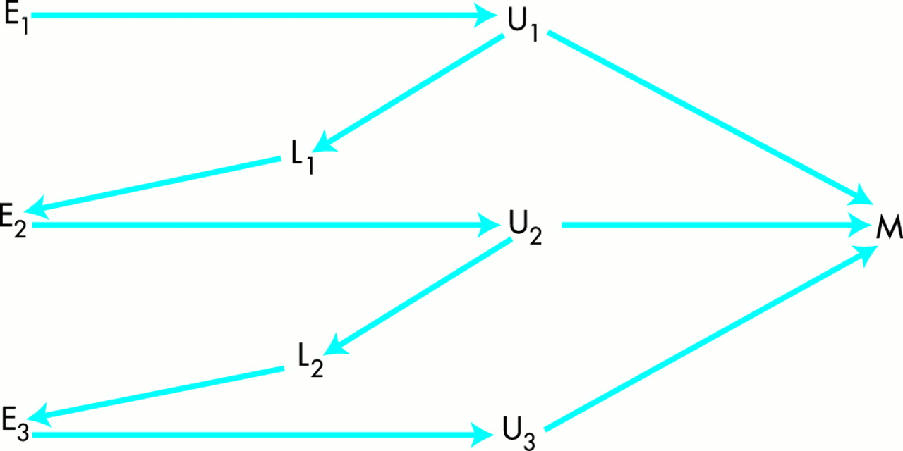
Figure 2 illustrates the relationships (1–3) for a hypothetical study of mortality rates (M). Exposure has been divided into three five year periods denoted by E1, E2, and E3; cumulative exposure (not shown) is defined simply as the number of years in employment. As before, an arrow from any variable to another implies that the former is a cause of the latter. U1, U2, and U3 denote occurrences of serious morbidity while employed in the three periods. As specified by (1), occurrence of morbidity during work is assumed to influence the decision to leave work—for example, U1→L1. For simplicity, it is assumed that leaving takes place at fixed time points only—5 years and 10 years after the start of exposure. As specified by (3), leaving work influences future exposure and hence cumulative exposure—for example, L1→E2. Finally, morbidity influences future mortality—for example, U1→M. In addition, this diagram assumes exposure effects: exposure is a cause of morbidity while employed—for example, E1→U1. A causal path linking exposure and mortality directly (for example, E1→M without passing through U1) might also have been added for realism but would not change the main message.
A causal diagram for a cohort study where morbidity during employment affects future employment and exposure. E1, E2, E3 denote exposure during years 1–5, 6–10, and 11–15, respectively. U1, U2, U3 denote unmeasured morbidity during employment in years 1–5, 6–10, and 11–15, respectively. M denotes mortality rate from selected cause. L1 and L2 denote presence or absence of employment at 5 years and 10 years, respectively. See text for further details.
One method proposed to overcome the attenuation problem is that employment status—for example, L1—be treated as a confounder.18 Morbidity—for example, U1—might seem a more obvious candidate but this is typically unobserved in historical cohort studies and employment status might be viewed as a very crude proxy measure of it. This solution will work18 only when there is no effect of exposure on morbidity. If there is an exposure effect—as postulated by fig 2—it will not. This can be deduced directly from the diagram: the existence of paths such as E1→U1→L1 violates condition C3a and thus standard adjustment for employment status is not warranted.
In fact this confounding problem does not appear to be solvable using standard statistical adjustment methods. Radically different methods, the so-called G methods,19,20 appear to succeed but, unfortunately, these are not currently available in standard statistical software. One exception is a G method recently implemented in the STATA statistical package. For the present, use of causal diagrams is recommended to explore the implications of various assumptions about the effects of health related selection out of the workforce.
Confounding and confounders in case–control studies
The definitions in boxes 1 and 2 apply as much to case–control studies as to cohort studies. Despite their design, the underlying causal question in the former concerns differences between exposure groups and therefore the question of confounding concerns the comparability of exposure groups, not the comparability of cases and controls. Consider a case–control study of lung cancer which is nested within an occupational cohort. The cohort (n = 2000) consists of both exposed and unexposed subjects, but it is too expensive to estimate exposure for all of them; instead all cases of lung cancer in the cohort (n = 50) and a random sample of non-cases (n = 200) are chosen for investigation of past exposure. The choice of case–control design here is a matter of practicality; it does not change the fact that confounding is a question of the comparability of exposed and unexposed members of the cohort.
In community based case–control studies also, confounding is a question of the comparability of exposed and unexposed members of the underlying study population (the study base). Modern teaching on case–control studies stresses the importance of defining this study population; it consists of all those people who would have been included in the case group if they had developed the disease.8 For example, in a case–control study based on lung cancer cases identified from a cancer registry, the study population might be roughly equal to the whole population of the region covered by the cancer registry. Confounding would refer to the comparability of the exposed and unexposed members in the whole of this region.
In searching for confounders among measured factors in a case–control study, a specific problem is that all of the study population has not been measured: only the cases and a sample of non-cases (controls). This is merely a problem of precision, in that a sample gives less precise information than a whole population. More importantly, to assess the comparability of exposed and unexposed in the study population, exposed and unexposed subjects in the control group only should be compared. This is because, roughly speaking, the controls in a case–control study represent the study population.8
Much of the present understanding of the confounding/selection problems associated with the healthy worker hire effect and healthy worker survivor effect has come from cohort studies. These problems are rarely mentioned in case–control studies but they are no less relevant. To see this, consider again the example of a case–control study nested within a cohort. In the cohort as a whole, healthier workers may have been selected into exposed jobs and ill workers may have been more likely to leave employment; these processes do not disappear simply because the researcher has chosen a case–control design. In theory the strategies adopted to deal with these problems in cohort studies could also be applied in nested case–control studies. For example, in one nested case–control study of shift work and cardiovascular disease, the authors adjusted for an apparent “healthy shiftworker hire effect”.
In community based case–control studies, the task of accounting for selection effects is far more complex given that subjects may have moved into and out of several different workplaces. As a simple attempt, it has been proposed6 that cases and controls should be classified into at least three categories—exposed workers, unexposed workers, and unemployed—with only exposed and non-exposed workers contributing to the analysis.
Confounding and selection bias in environmental epidemiology
Understanding of health related selection, and how it contributes to confounding, is well developed in occupational epidemiology. In environmental studies, analogies with occupational selection effects may be informative. Exposed groups are sometimes defined by geographical residence—for example, proximity to a suspected environmental pollutant; confounding due to selection bias, over and above general socioeconomic confounding, is also possible here. An effect analogous to the healthy worker hire effect could occur if a cohort of residents were compared with the general population, as from the time they moved into the area. If moving to a new house (mobility) is associated with better health status then there might be a “healthy mover effect” with morbidity or mortality rates lower initially than in the general population. For the same reason, a long duration of residence at the same address might be associated with reduced mobility as a consequence of poor health. In theory this confounding, which one might also call an “unhealthy stayer effect”, could create a false dose response relationship.
Box 3: key points
-
The notion of confounding as non-comparability is unambiguous, but there is no simple, completely foolproof definition of a confounder
-
There have been recent changes in the necessary conditions for a confounder: factors affected by exposure are not confounders
-
There can be a conflict in the notions of confounding as non-comparability (box 1) and as non-collapsibility. The non-comparability definition is preferable
-
For identification of confounders:
data is generally an imperfect guide
causal diagrams can help clarify thinking
external evidence may be relevant
degree of confounding is more important than statistical significance
-
In occupational health:
the healthy worker hire effect (HWHE) and survivor effect (HWSE) can be construed as confounding
both HWHE and HWSE can affect within-cohort comparisons
the HWSE leads to attenuation of exposure–response relationships based on cumulative exposure
health related selection into and out of work is also relevant in case–control studies
QUESTIONS (SEE ANSWERS ON P 164)
For each question please indicate which answers are true or false.
Confounding:
arises from lack of comparability of exposed and unexposed groups
arises from lack of comparability of cases and controls in case–control studies
is not a concern when comparing groups with different degrees of exposure
is not a concern in descriptive (non-causal) studies
Confounders:
are risk factors for disease
will always show a relationship with disease risk in data
must be significantly different (p < 0.05) between exposed and unexposed groups
must not be caused by exposure
A change in estimate definition of a confounder:
is based on a comparison of adjusted and unadjusted measures of exposure effect
may sometimes conflict with the criteria C1–C3a
is defined solely in terms of statistical criteria
Causal diagrams:
distinguish between association and causation
have different forms depending on whether odds ratios or incidence rate ratios are used
can help to decide whether a suspect factor is a confounder
The healthy worker hire effect and healthy worker survivor effect:
are examples of selection bias
are not examples of confounding
can affect dose–response relationships
do not affect data from case–control studies
In comparisons of worker groups defined by cumulative exposure:
duration of employment and cumulative exposure may be correlated
duration of employment and health will be associated if there is a healthy worker survivor effect (HWSE)
the “dose–response” relationship may be exaggerated because of the healthy worker survivor effect (HWSE)
REFERENCES
Supplementary materials
Confounding and confounders
R McNamee
Web-only References
[View PDF]
On causes:
Neyman J. Sur les applications de la thar des probabilities aux experiences Agaricales: essay des principles. Transl. D Dabrowska, T Speed in Statistical Sciences 1990;5:463-472.Lewis D. Causation. J Philos 1973; 70:556-67.
.
Rubin DB. Estimating causal effects of treatments in randomized and non-randomized studies. J Educ Psych 1974;66:688-701.Rothman KJ. Causes. Am J Epidemiology 1976;104:587-92.
Sobel MS. Causal inference in the social sciences. J Am Statist Assoc 2000; 95:647-651.
On adjusting for pregnancy history:
Nurminen T. On adjusting for the outcome of previous pregnancies in epidemiologic reproductive studies. Epidemiology 1994;6:84-86.Weinberg C. Should we adjust for pregnancy history when the exposure effect is transient? (Letter) Epidemiology 1995;6:335-336.
Nurminen T Should we adjust for pregnancy history when the exposure effect is transient? (Reply) Epidemiology 1995;6:336-337.
On selection effects in occupational cohorts:
Fox AJ, Collier PF. Low mortality rates in industrial cohort studies due to selection for work and survival in the industry. Br J Prev Soc Med 1976;30:225-230.McMicheal AJ. Standardised mortality ratios and the �healthy worker effect�: scratching beneath the surface. J Occup Med 1976;18:165-168.
Wen CP, Tsai SP, Gibson RL. Anatomy of the healthy worker effect: a critical review. J Occup Med 1983;25:283-289.
Sterling TD, Weinkam JJ. Extent, persistence and constancy of the healthy worker or healthy person effect by all and selected causes of death. J Occup Med 1986;28:348-353.
Monson RR. Observations on the healthy worker effect. J Occup Med 1986;28:425-433.
On collapsibility definition of a confounder:
Whittemore AS. Collapsing multidimensional tables. J R Stat Soc B 1978;40:328-340.Boivin JF, Wacholder S. Conditions for confounding of the risk ratio and of the odds ratio. Am J Epidemiology 1985;121:152-158.
Grayson DA.. Confounding confounding. Am J Epidemiology 1987;126:546-63.
Greenland S, Morgenstern H. Poole C, Robins JM. Re: �confounding confounding�. (Letter). Am J Epidemiology 1989;129:1086-9.
Grayson DA.. Re: �confounding confounding�. (Reply). Am J Epidemiology 1989;129:1089-1091.
On control of the healthy (shift)worker hire effect in case-control studies:
McNamee R, Binks K, Jones S, Slovak A, Cherry NM. Shiftwork and mortality from ischaemic heart disease. Occupational and Environmental Medicine 1996;53:367-373.
On control of the healthy worker survivor effect and similar problems:
Hertz-Picciotto, Michael Arrighi H, Suh-Woan H. Does arsenic exposure increase the risk of circulatory disease? Am J Epidemiology 2000;151:174-181.Steenland K, Deddens J, Salvan A, Staynew L. Negative bias in exposure-response trends in occupational studies: modelling the healthy worker survivor effect. Am J Epidemiology 1996;143:202-210.
Robins JM, Blevins D, Ritter G, Wulfson M. G-estimation of the effect of prophylaxis therapy for pneumocystis carinii pneumonia on the survival of AIDS patients. Epidemiology 1992;3:319-336.
Robins J. A new approach to causal inference in mortality studies with a sustained exposure period: application to control of the healthy worker effect. Math Modelling 1986;7:1393-1512.
Sterne J, Tilling K. G-estimation of causal effects, allowing for time-varying confounding. The Stata Journal 2002;2:164-182