Article Text

Statistics from Altmetric.com
Introduction
Selection of study subjects from restricted source populations according to prespecified criteria is an approach that is frequently used in cohort studies. The purposes of such restrictions are to enhance study feasibility and to increase the prevalence of exposure or the completeness of follow-up, thereby increasing study validity and precision. Typically this may involve recruiting participants from a subgroup of the general population, rather than sampling directly from the entire general population. Such subgroups may be defined on the basis of occupation, gender, geographical area, birth cohort, etc. The British Doctors' Study1 and the Nurses' Health Study,2 occupational cohorts,3 follow-up of participants in specific events,4 analyses restricted to specific subgroups of the population, such as non-smokers,5 ancillary analyses of non-randomised exposures in randomised studies,6 and follow-up studies of screening attendants7 are all examples of cohort studies based on restricted samples.
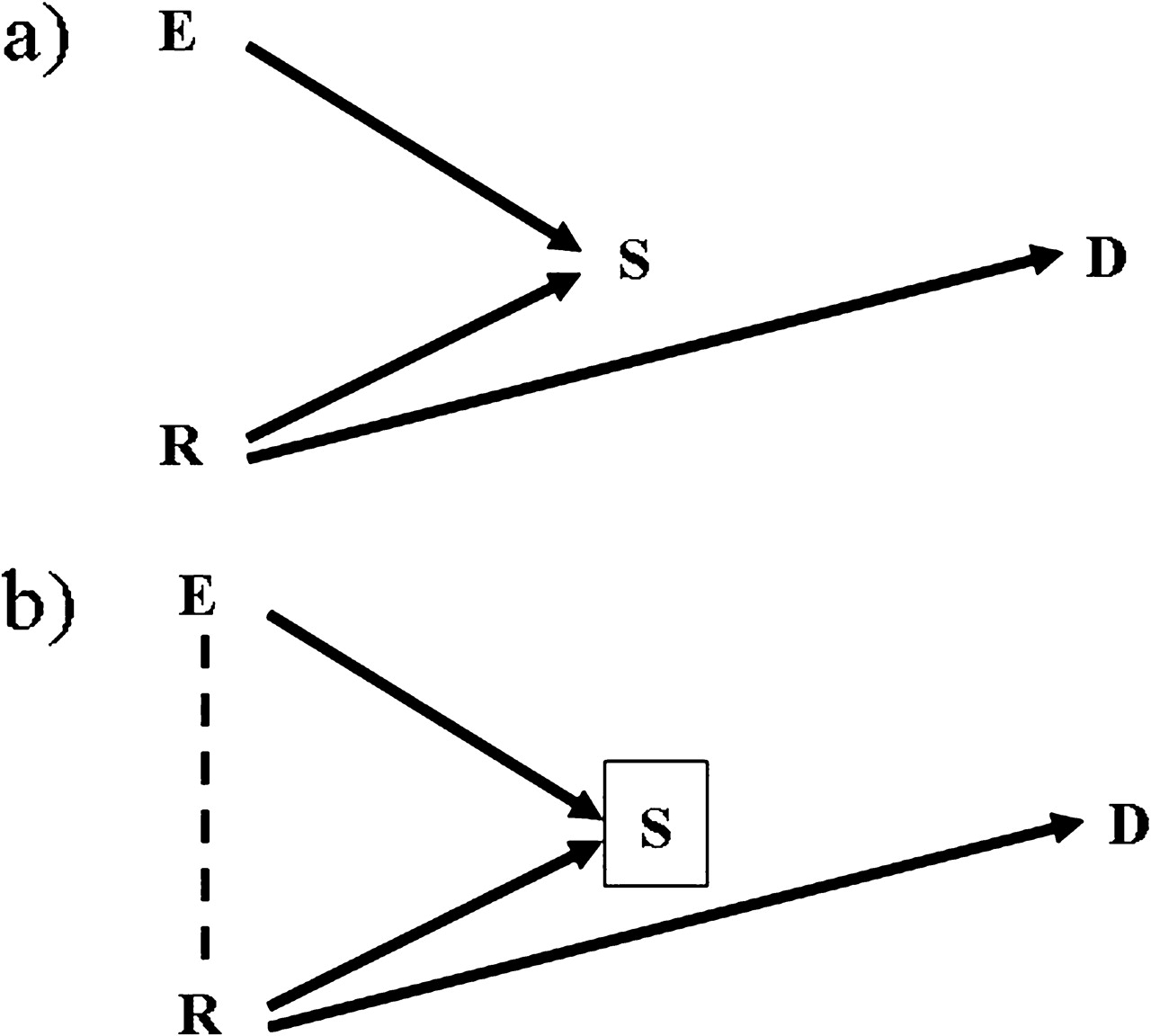
Undoubtedly, restriction of the source population may introduce problems of generalisability of the study findings, but this also applies to studies that are based on the general population (eg, most cardiovascular epidemiology involves cohort studies in specific communities rather than true general population samples). We will therefore not consider issues of generalisability here; rather, our focus is on whether using a restricted source population may affect the validity of the exposure–disease associations.8 9 In particular, bias will be introduced if a risk factor for disease is not associated with exposure in the general population but is associated with exposure in the study population, as a result of the selection process. Such biases can be represented using directed acyclical graphs (DAGs).8 10–13 The example depicted in figure 1A represents a population in which there is no association between an exposure (E) and a disease (D); there is another risk factor (R) for the disease, but this is not a source of confounding as it is not associated with the exposure. However, E and R both affect the likelihood of being selected (S=1) into the study. When analyses are restricted to the selected subjects, there is an inherent conditioning on S (as represented by a square around S in figure 1B), which leads to a spurious association between E and R (represented by a dashed line). Under this scenario, even if E has no causal effect on D, the backdoor path E–R–D is opened and the estimated associational RR between the exposure and the disease (ARRDE) may differ from the causal RR (CRRDE). This could, for example, be the situation in a cohort study of the effect of obesity (E) on breast cancer (D) based on breast cancer screening participants (the restricted source population). In this example, obese women (E) are less likely to attend the screening programmes,14 while women with a family history of breast cancer (R) are more likely to participate. Among those who attend screening (ie, conditioning on those with S=1), obesity (E) and family history of breast cancer (R) become positively correlated. In fact an obese woman is more likely to have a family history of breast cancer within the selected sample than in the general population, because otherwise she may not have participated in the screening programme. As a result, family history of breast cancer is a confounder of the obesity–breast cancer association if studied among screening attendees, but is not—or to a lesser extent—in the general population.

Diagram of a cohort based on a selected sample. (A) In the population the exposure of interest (E) is not associated with the disease of interest (D) that is caused by a risk factor (R). Both E and R affect the probability of being selected (S) as a member of the cohort. (B) The study is carried out in the selected sample, and therefore there is an inherent conditioning on S (a box around a variable means conditioning for that variable) which generated an induced association between E and R (represented by a dashed line).
This type of bias has been extensively discussed in the causal inference literature from a theoretical point of view.8 9 Hernan and colleagues' 2004 paper on selection bias provides the conceptual framework and indicates that if the risk factor associated with the selection process is known and measured, it is possible to adjust for selection bias, whereas if the risk factor is unmeasured, the effect estimates may be biased. However, although the theoretical basis of selection bias is clear, there have been few attempts to quantify the likely strength of such biases. One exception is that of Greenland,15 who studied the setting of figure 1B with dichotomous exposure and outcome variables, employing methods originally developed to quantify the impact of unmeasured confounding.16 He calculated the likely maximum strength of the bias in the estimation of the E–D association in the S=1 stratum as a function of the ORs corresponding to the true associations depicted in figure 1B (ie, ORSE, ORSR, ORDR). However, it is not clear how these results apply to cohort studies. Because of the increasing frequency of cohort studies based on selected populations, such as the internet-based birth cohort studies based in Italy (NINFEA cohort) and New Zealand (ELFS),17 quantifying the potential biases involved in analysing such data is timely and relevant.
Our aim is therefore to study the extent of these biases. We use simulations to mimic a variety of cohort restrictions and disease settings and examine the consequent bias in the estimated exposure hazard (or rate) ratio (HR) of disease. We then discuss these results in terms of whether, and under what circumstances, the resulting selection bias is serious enough to strongly bias the exposure effect estimates. For simplicity, we will assume throughout the paper that there is negligible random variation, that all variables are measured without error, and that there is uninformative censoring.
Sample selection and disease risk factors
As previously recognised,9 18 a fundamental characteristic of selection bias in restricted cohort studies is that the selection process makes a disease risk factor, which may not be associated with the exposure in the general population, become associated with the exposure among the study population and therefore act as a confounder.
Confounders in the general population and risk factors that become confounders in a restricted source population are usually indistinguishable when the study is analysed. Although typically some disease risk factors (ie, potential confounders) are known a priori, it is seldom known whether these are associated with the exposure of interest in the specific population in which the study will be carried out. Both in general population-based and restricted cohorts, therefore, researchers attempt to collect information on all known and suspected important risk factors of the disease in the population that they are studying, regardless of their expectations about whether these are associated with the exposure or not. The example of the association between smoking and socioeconomic position (SEP) illustrates this point well. Depending on the population and the calendar period, SEP can be positively or negatively associated, or not associated at all, with smoking. Researchers aiming to estimate the association between smoking and mortality will always attempt to collect information on SEP and, in most instances, will control for it, irrespective of whether the confounding effect of SEP is due to a real association between SEP and smoking in the general population or a spurious association caused by the sample selection process.
Another possible consequence of the selection mechanism is a change in magnitude, and in extreme cases direction, of the confounding effect of a risk factor. This may occur if the strength of the association between the risk factor and the exposure in the selected sample differs from that originally present in the general population. For example, when two (parent) variables influence a third (child) variable in the same direction, conditioning on the child variable likely leads to a negative association between the parent variables.8 Thus, if an exposure and a confounder influence the selection process in the same direction, the original association between exposure and confounder will be reduced in the subset of those who participate if they were originally positively associated, or increased if their original association was negative. For example, in many populations smoking and physical exercise are negatively associated. In a hypothetical study restricted to blood donors, who typically have a healthy lifestyle and thus smoke less and exercise more than the average individual in the general population, the sample selection would add a positive association between smoking and physical exercise. Therefore, the original negative association present in the general population would be, if anything, attenuated among blood donors.
In the next section, we use simulations to quantify the likely extent of selection bias arising from the use of restricted cohorts.
Quantification of the bias
Methods
We conducted Monte Carlo simulations of alternative settings corresponding to the scenario of figure 1B to quantify the resulting bias in the estimation of the E–D effect when conditioning on S=1 and not adjusting for R.19 The generation process of the four variables of figure 1B is described below.
We generated E and R as marginally independent binary variables, with prevalence, respectively PE and PR, initially set equal to 0.5 in the source population. They were later allowed to decrease to 0.25 for PE and to 0.1 for PR, in order to investigate scenarios more frequently addressed by epidemiologists.
The binary variable S was generated using a logistic regression model with baseline prevalence, PS, equal to 0.5 and with the ORs for the explanatory binary variables E and R taking values 0.25, 0.33, 0.50, 2, 3 and 4. Specifically, with αS indicating the log(odds) of S=1 among the non-exposed, βSE indicating the log(OR) corresponding to exposure E and βSR indicating the log(OR) corresponding to R, the generating model was:
A more complex model that included an interaction term between E and R was also considered:
with ORinter, corresponding to exp(βinter), set at values 0.5 or 2. The interaction term was introduced to examine more realistic selection settings. For example, in the first empirical demonstration of Berkson's bias, Roberts and colleagues found that not only do chronic conditions increase the chance of hospitalisation, but they often also interact more than multiplicatively.20
We generated time to the outcome D assuming a constant rate λ—that is, we assumed that time to event followed an exponential distribution.21 The baseline rate λ0 was set equal to 0.01, 0.03 or 0.06 events/year, with administrative censoring time set at 5 years. The rate λ was allowed to be affected only by R, with HRDR taking values 0.25, 0.33, 0.50, 2, 3 and 4, while we assumed no E–D association—that is, HRDE=1. Specifically, with βDE indicating the log(HR) of D for the exposure E and βDR indicating the log(HR) of D for the risk factor R, the log rate function for D, log(λ), was defined as:
with βDE fixed at 0.
We generated a total of 1000 Monte Carlo simulated datasets of 5000 subjects for each combination of the parameters described above. We also used a size of 2500 subjects, increasing the number of simulations (n=2000), to deal with the greater impact of random variation.
In each simulated dataset, we estimated two main parameters in the stratum S=1 (which sample size varies as a consequence of the selected parameters for the selection process): the association between E and R (ORER) and the association between E and D (HRDE) which is induced by the selection process. The estimate of HRDE was obtained fitting a Cox proportional hazards regression model with no adjustment for R.22 We then calculated the bias in the E–D association as the difference between zero, that is the true value of βDE, and the logarithm of the estimated HRDE. For each scenario, we summarised the bias, and the estimated values of βDE, in terms of means, SD, and 5th and 95th percentiles.
Results
We first considered the situation with prevalence of E and R both equal to 0.5, ORinter=1 (ie, no multiplicative interaction), and λ0=0.03 (the ‘reference scenario’ in table 1). As expected, the size of the bias in the estimation of ORDE depended on: (i) the induced association between the exposure and the risk factor (ORER), which increased in absolute terms with the absolute size of ORSR and ORSE; and (ii) the magnitude of the association between the risk factor and the disease (HRDR). The largest values of the bias in the log OR were ±0.15 (table 1, ‘reference scenario’), which were reached when ORSE, ORSR and HRDR were furthest from the null value (ie, equal to 0.25 or 4). Note that in table 1 the range for log(ORER|S=1) is not symmetrical because the magnitude of the association induced by the selection between E and R also depends on the prevalence of S in the population (Ps), with the strongest association obtained when Ps=0.5. Supplementary table 1 presents the complete results for all combinations of the values of ORSE, ORSR and HRDR. The mean bias decreased from ±0.15 to just ±0.02 when the three ORs/HRs were equal to 2 or 0.5.
Bias in the crude estimation of the E–D association by selected values of the data generating parameters; results from 1000 simulations
When an interaction term between E and R was included in the model generating S, the induced E–R association increased considerably (figure 2), up to a log(OR) of −0.98 (table 1, row 2) when ORSE and ORSR were equal to 0.25 and the ORinter was 0.5. The bias increased accordingly, ranging from −0.24 to 0.27 (table 1, row 2). This situation is equivalent, in terms of induced bias, to those involving very strong marginal associations with selection. It is clear from figure 2 that the impact of the interaction is not the same for all the parameter combinations, as the magnitude of the induced E–R association is strengthened or reduced according to the sign of the interaction term but also to the size of the stratum of subjects exposed to both E and R.

Mean OR of the induced E–R association in the stratum of those selected (S=1) by selected values of the association of the exposure (ORSE) and the risk factor (ORSR) with the selection process and of the E–R interaction (ORinter); results from 1000 simulations.
Neither the prevalence of the exposure E (table 1, row 3) nor the baseline rate for the disease D (table 1, rows 4–5) or the sample size (table 1, row 6) affected the extent of the bias. Conversely, the prevalence of R, which becomes a confounder of the E–D association when S=1, had a non-marginal effect. For a given value of the induced E–R association, the bias reached its peak when the prevalence of R among the selected subjects (S=1 stratum) was 0.5. For this reason, when the population prevalence of R was set equal to 0.1 instead of 0.5, the range of the mean bias decreased to (−0.12; 0.07) (table 1, row 7).
Discussion
Conducting cohort studies in a restricted sample of the general population may offer several advantages, including more precise measurement of the exposure, higher exposure prevalence, enhanced feasibility of the study, better control of confounding, increased sample size, higher recruitment rates, and a higher completeness of follow-up. These advantages should be balanced against issues of validity.
In this paper we have shown, via simulations, that the possible bias introduced by restriction of the source population is usually weak when internal comparisons are carried out within the cohort, with a maximum bias in the log(HR) of ±0.15.
These results are in agreement with those of Greenland,15 who used an analytical approach to quantify the maximum selection bias in settings where the outcome risk is rare so that the analysis of cohort data can be performed using logistic regression. Our simulations add further insight to these results as we examined a wide range of disease and selection parameters, including exposure and risk factor prevalence, which highlighted their individual role in influencing the extent of the bias. Further, we considered settings where exposure and risk factor interact when influencing the selection process. Some additional points are warranted.
First, the bias is necessarily small when the association between the exposure of interest and the selection process is relatively weak (ie, 0.5<OR<2). In particular, when the exposure-selection OR is equal to 2 or 0.5, while the risk factor-selection OR and the risk factor-disease HR are allowed to take values up to 4 or down to 0.25, the maximum bias in the estimated exposure–disease association is within the ±0.07 range (on the log hazard scale). For example, consider the Million Women Study, a cohort nested within the breast screening programme in the UK.7 From the study carried out to compare the characteristics of the study participants with the rest of the population (women who attended the screening but did not join the study plus not attendants),23 the participation OR for current use of hormone replacement therapy, which is the main exposure of interest of the study, was derived. This estimated OR was about 1.6. On the basis of this information it is possible to assume that, in this cohort, the bias introduced by the baseline selection on the estimates of the effect of hormone replacement therapy on the outcome of interest would be negligible.
Second, selection must be associated with one or more unmeasured or unknown disease risk factors in order to introduce bias. However, unknown or unmeasured disease risk factors can introduce bias whether or not the cohort is based on the general population or a restricted source population; in the latter case, the sample selection can either increase or decrease the overall bias, with a magnitude and direction difficult to predict if there are multiple risk factors involved.24
Third, we have shown that even when all of the associations involved in the selection and outcome mechanisms are reasonably large (eg, all ORs/HRs of 4.0 or 0.25), the prevalence of the risk factor R is about 50% and there is no adjustment for R, the resulting bias is relatively weak (ie, ±0.15 on the log scale). This is reassuring, as this scenario is rather extreme and very unlikely to occur in practice. Besides, a disease risk factor with a 50% prevalence and a disease HR of 4.0 would have an attributable fraction of 60% and is therefore unlikely not to have been known and measured when a study is planned.
The scenarios considered in our simulations were restricted to binary exposure and binary risk factor and assumed no association between the exposure and the risk factor in the general population. A limitation is that we examined only the case of a single unmeasured determinant of the disease that also influences the selection process. However, we believe it is unlikely that multiple and independent important disease risk factors would affect the sample selection. It is indeed reasonable to consider R as a vector resulting from the combination of a set of correlated risk factors, all moderately associated with S. Finally, we only showed the findings derived from the analyses based on the assumption of a null causal association between the exposure and the outcome of interest; however choosing a true associational value, βDE, different from zero would not modify the simulation results and therefore our conclusions.
We conclude that using a restricted source population for a cohort study will, under a range of sensible scenarios, produce only weak bias in estimates of the exposure–disease associations. On the other hand, the use of such restrictions may increase the response rate and the exposure prevalence, as well as being the only feasible approach in many circumstances.
What we already know on this subject
Baseline selection of participants in cohort studies may affect the study validity.
This happens when, because of the selection process, the confounding effect of an unknown or unmeasured disease risk factor is larger in the selected sample than in the general population.
What this study adds
We conducted Monte Carlo simulations to quantify the likely extent of the selection bias affecting the exposure-disease association, varying all the parameters involved: prevalence and effects of exposure and risk factor on both the selection and outcome process, selection prevalence, baseline incidence rate of the outcome and sample size.
The maximum bias is relatively weak (±0.15 in the log Hazard Ratio scale). When scenarios typically seen in epidemiological studies were considered the bias in the log Hazard Ratio drops to ±0.02.
References
Supplementary materials
Web Only Data jech.2009.107185
Files in this Data Supplement:
Footnotes
Funding The study was conducted within projects partially funded by Compagnia SanPaolo/FIRMS, the Piedmont Region, the Italian Ministry of University and Research (MIUR), the Italian Association for Research on Cancer (AIRC) and the Massey University Research Fund (MURF). The Centre for Public Health Research is supported by a Programme Grant from the Health Research Council of New Zealand.
Competing interests None.
Provenance and peer review Not commissioned; externally peer reviewed.