Article Text

Abstract
OBJECTIVE To develop a chart to identify non-familial short stature.
DESIGN A height chart that adjusts for maternal, paternal, midparental, or sibling height based on the British 1990 height reference.
MAIN OUTCOME MEASURE Height between 2 and 9 years of age.
RESULTS The chart identifies children whose height is below the familially adjusted 0.4th centile, assuming a correlation of 0.4 between child height standard deviation score (SDS) and familial height SDS. The adjustment can be for parents, either alone or together, or for a sibling aged 2–9 years. The chart identifies about 2 children/1000 over and above the 4/1000 identified by the unconditional 0.4th centile.
CONCLUSION The chart should be a useful addition to screening programmes for short stature.
- short stature
- midparental height
- growth chart
- screening
Statistics from Altmetric.com
Screening for short stature in childhood is useful for identifying growth disorders such as growth hormone deficiency or Turner's syndrome. However, as with any screening instrument its performance needs to be quantified.1 The UK height reference2 ensures a low false positive rate because its 0.4th centile screens in only four children/1000, but the corresponding sensitivity is poor.1 In particular, short children of tall parents are likely to be missed.
Midparental height, the average of the two parents' heights, is the traditional approach to adjusting for family size. Target height, derived from midparental height by adjusting for the child's sex, predicts the child's height as an adult. A recent paper3investigated target height in a Swedish growth study, but target height has been criticised4 because it does not adjust for regression to the mean.
An alternative use of midparental height is to relate it directly to the child's current height, which avoids the concept of target height in adulthood. Tanner and colleagues5 published a chart that adjusts child height, expressed as a centile, for midparental height, and so identifies children who are short within their family. This more direct approach is preferable, because it focuses on the child's height now rather than as an adult. It also adjusts for regression to the mean.
However, adjusting for midparental height is not entirely straightforward. It implies that very short children are of appropriate height if their parents are short, which might not be the case. What is needed is a combined approach, to identify not only very short children, irrespective of their parents' height, but also short children whose parents are tall.
A recent practical problem with midparental height is the single parent family, where only one of the two parents can be measured. However, it should be recognised that the height of one parent alone provides useful information about the child's height. In addition, adjustment can be made for sibling height if there is a sibling close enough in age. This also assumes, as does the midparental height adjustment, that the rest of the family does not suffer from a growth disorder.
To be able to deal with the various familial alternatives—one parent and/or the other, with or without a sibling—a modified form of familial height chart is needed to assess the index child's current height. This paper describes a simple chart that achieves this aim.
Methods
The relation between average child height and family height is conventionally summarised by the regression equation: child height = intercept + coefficient × midparental height which predicts the child's height from the midparental height. The intercept and regression coefficient are estimated by linear regression, but they depend crucially on the child's age; Tanner and colleagues5 fitted a separate equation for each year of age from 2 to 9 years.
If height is converted to a standard deviation score (SDS)—the number of standard deviations above or below the mean height for age and sex—then the age and sex effects are adjusted for and the regression equation simplifies to: child height SDS = coefficient × midparental height SDS (Equation 1).
Midparental height SDS is calculated as the mean height SDS of the parents, adjusted for assortative mating (appendix ). Applied to the reference population, the equation's intercept disappears, and the regression coefficient is the same as the correlation coefficient between child height SDS and midparental height SDS. This holds generally for pairs of variables that are related in SDS form.6 The correlation coefficient, unlike the regression coefficient of child height on midparental height, is effectively constant over the age range 2–9 years.7
Children whose height or height SDS is sufficiently low compared with their midparental height are identified as having non-familial short stature. The cut off point is set to some low centile from the distribution—for example, the second centile height, lying two residual standard deviations below the height predicted by the equation. An advantage of the height SDS regression equation (equation 1) is that the residual standard deviation can be calculated from the correlation coefficient. Therefore, the sole information required to identify non-familial short stature is the correlation coefficient between height SDS and midparental height SDS.
If this correlation coefficient is r, then applied to the reference population the residual standard deviation (RSD) is given by √1−r 2. The cut off point for unadjusted short stature is the 0.4th centile,2 so that any child whose height is below the 0.4th centile and unexplained should be investigated further. It is logical to use the same cut off point for familial short stature. The 0.4th centile corresponds to −2.67 SD, so that the 0.4th centile of child height SDS conditional on midparental height SDS is 2.67 RSD below the fitted regression line, and is given by the following equation: 0.4th conditional centile height SDS = r × midparental height SDS − 2.67 √1−r 2 (Equation 2).
The value of r, the correlation between child height and midparental height, is obtained from the literature.
Equations 1 and 2 apply generally to any pair of variables that are in SDS form,6 so that the SDS of midparental height can be replaced by height SDS for either parent alone, or for the child's sibling.
Results
Himes and Roche7 compared the correlations between height and midparental height at different ages in four different studies, and showed that for children in the age range 2–9 years they were effectively constant within each study, with values between 0.4 and 0.55. They were calculated for heights in annual age groups, and so are broadly equivalent to correlations for height SDS and midparental height. Because midparental height does not change with age, its correlation with child height is the same whether or not it is in SDS form. Thus, the correlations of 0.40–0.55 between child height and midparental height apply equally to child height SDS versus midparental height SDS. Tanner's midparental height standard5 was based on correlations of 0.53 for boys and 0.49 for girls.
For illustration, assume a relatively low value of 0.4 for the correlation. Figure 1 shows a graph of child height versus midparental height (both in SDS units), and the midparental conditional 0.4th centile line (equation 2) with a slope r of 0.4 superimposed. The unconditional 0.4th centile also appears as a horizontal dotted line. The two centile lines delineate three regions below them, labelled A, B, and C in fig 1. Regions A and B are below the unconditional 0.4th centile and, under current screening recommendations,1 children with heights in either of these regions should be referred. The difference between them is that in region A the child's height is appropriate for midparental height—it is above the conditional cut off point—whereas in region B it is not. Region C contains children, nearly all of above average midparental height, who despite being above the unconditional 0.4th centile are nevertheless very short for their midparental height—that is, below the conditional 0.4th centile. It is this region that is important for the midparental height adjustment; without it children cannot be identified as unusually short within their family.
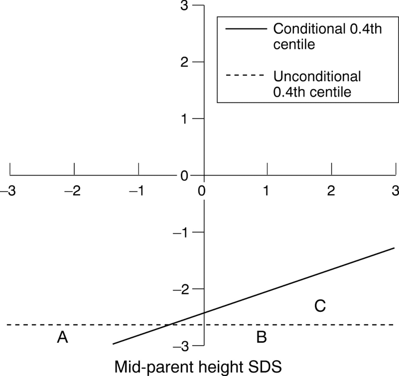
Child height standard deviation score (SDS) adjusted for midparental height SDS assuming a correlation of 0.4, showing the conditional 0.4th centile (solid line) and unconditional 0.4th centile (dotted line). Three regions labelled A, B, and C lie below the two centiles (see text for details).
Figure 1 adjusts child height for midparental height. A similar chart can be constructed to adjust for the height of either parent alone, simply by altering the correlation coefficient—the slope of the conditional 0.4th centile. It can be shown on theoretical grounds that the height SDS correlation for a child with either parent alone should be 0.8 times the midparental height correlation (appendix ). Therefore, if the midparental correlation is 0.40, then the single parent correlation ought to be 0.32. This is low compared with the value of 0.5 predicted from genetic theory.8
The chart in fig 1 can also be applied to siblings close in age to the index child. In theory, the height correlation between siblings ought to be 0.5,8 the same as the parent–child correlation. Data from the Fels study8 show that unlike the parent–child correlation the sibling–sibling correlation is close to this value. For children at each year of age between 2 and 9 years, the height correlation with siblings when they were at the same age is 0.45–0.52, whereas the correlation with each parent alone is only about 0.30.
This poses a problem—the slope of the family conditional centile is 0.40–0.55 for midparental height, 0.30–0.32 for parental height, and 0.45–0.52 for sibling height. Does this mean that different charts are needed for each combination?
Figure 2 is an extension of fig 1, which shows three different conditional 0.4th centiles representing correlations of 0.3, 0.4, and 0.5. The unconditional 0.4th centile is also shown labelled “r = 0”. A sample of 1000 randomly generated points based on a correlation of 0.4 is superimposed, representing a population of normally growing children. The two scales are labelled to reflect the nine centile format of the UK 1990 reference,2 on which the chart's design is based.

A plot of 1000 randomly generated points with correlation 0.4, along with the unconditional 0.4th centile (labelled “r = 0”) and conditional 0.4th centiles for correlations 0.3, 0.4, and 0.5.
Figure 2 emphasises the extreme nature of the 0.4th centile—all the centile lines are far from the main body of data. There are four points on or below the unconditional 0.4th centile (regions A and B), which by chance is exactly the expected number, four/1000. In addition, depending on which line is used, there are between two and five points below the conditional centile (regions B and C), again similar to the expected number of four. The important part of fig 2 is region C, below the conditional centile but above the unconditional centile, indicating children who are identified with a familial adjustment but who are missed by the simpler screen. The shape of region C is defined as the triangle with the conditional centile above and the unconditional centile below, and so is different for each of the conditional centile lines.
Two of the points below the conditional centile are also below the unconditional centile (in region B), so these are children who would be screened in anyway. There are just three further children who would be identified only with the conditional centile, one belowr = 0.4 and two more belowr = 0.5. The theoretical “screen in” rate in region C, assuming a bivariate Gaussian distribution, is just under two/1000, whichever conditional centile line is used.
Thus, there is little to choose between the different conditional centiles, and the middle line is a reasonable compromise for all three roles: midparent, single parent, and sibling. Figure 3 shows how the three adjustments can be provided in a single chart.
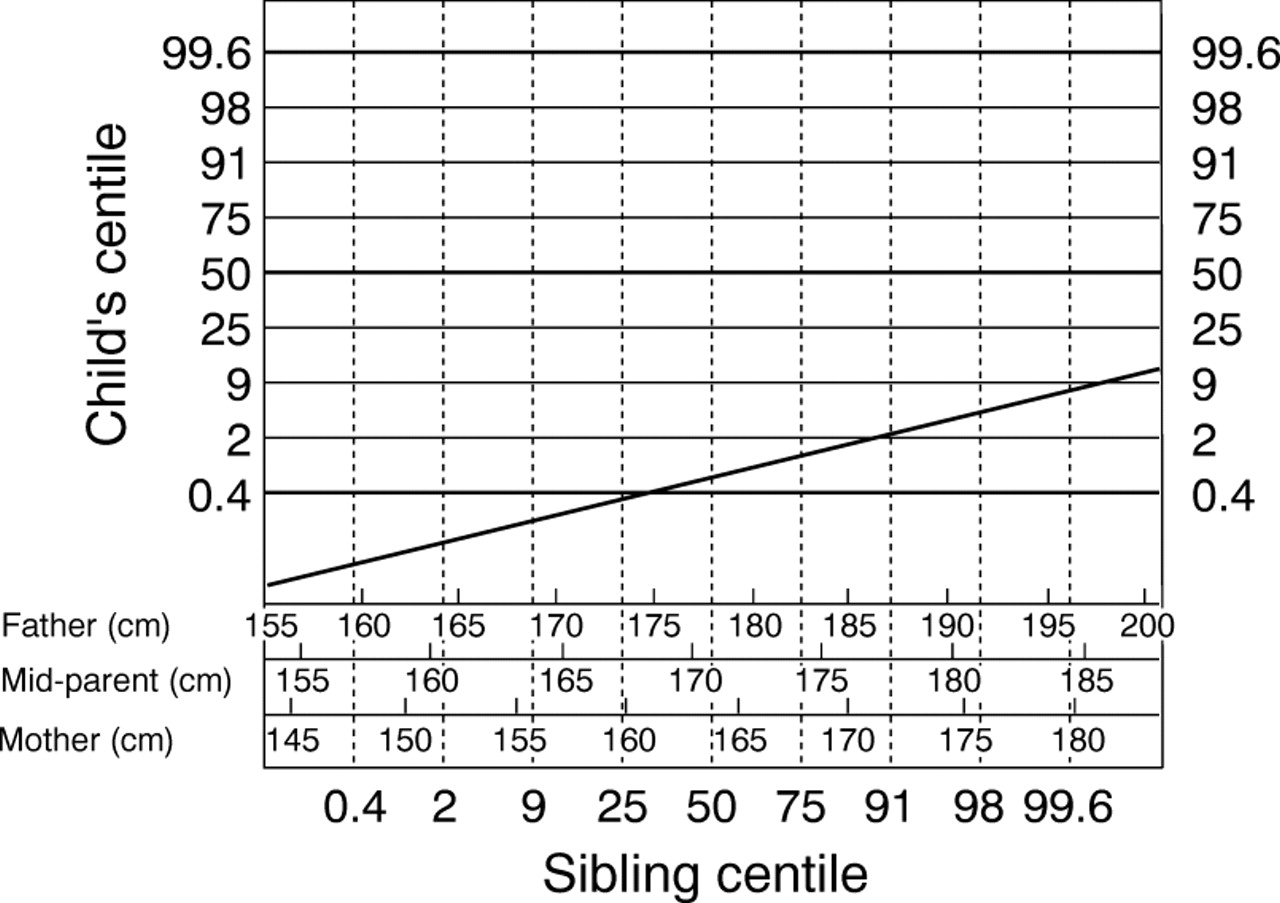
A family height chart to adjust for midparental, single parent, or sibling height. The index child and sibling are plotted as height centiles obtained from a reference centile chart.
The chart is constructed as follows: the single parent height scales convert height to an SDS using the UK 1990 reference data for age 22.2 For the midparental height scale, height SDS for the two parents cannot be averaged to obtain midparental height SDS,9 and a compromise solution is described in appendix. The sibling height scale is simply the centile as read off the height chart.
To use the chart, the index child's height is first plotted on a reference centile chart to obtain the height centile band. To adjust for the height of father or mother alone, the child's centile is then plotted against the parent's height (in cm) using the appropriate scale. To adjust for midparental height, it first needs to be calculated by averaging the heights of the two parents, then the index child's centile is plotted against midparental height on the chart using the midparental scale. Note that midparental height not target height is used, so there is no sex adjustment. To adjust for sibling height, the sibling needs first to be plotted on a centile chart to obtain the height centile band, then the index child's centile is plotted against the sibling's centile.
In each case, if the index child's point lies below either the unconditional or conditional 0.4th centile line then the child should be referred.
Discussion
This paper shows how the height of children aged between 2 and 9 years can be adjusted for the height(s) of other family members to identify children with non-familial short stature. As well as the conventional midparental height adjustment, the chart (fig 3) also provides an adjustment for the height of either parent alone, or of a sibling of similar age to the index child.
The chart adjustment, if implemented universally as part of a screen at school entry, ought to identify about two children/1000 over and above the four/1000 that the 0.4th centile currently picks up. This is not a large number. In addition to these false positive short normal children there will be some “true” positives who are very short within their families. In the Wessex growth study,10 27 children below the third centile of the Tanner standard had pathology, and six of these children were above the 0.4th centile of the UK 1990 reference. One of the six was below both the paternal conditional and the midparental conditional 0.4th centile, so that use of the conditional centile increased the sensitivity slightly from 77.8% (21 of 27) to 81.5% (22 of 27).
For siblings, although hard data are lacking, there is persistent anecdotal evidence of children in tall families being identified by parents as short solely through comparison with their younger and relatively taller sibling(s).
The way to use the chart as part of a universal screen is as follows. The nurse should measure the child and plot his/her height on the conventional centile chart. If it is above the ninth centile then the child is fine and will not need to be measured again. The ninth centile is relevant because no child above it can at the same time be below the conditional 0.4th centile, whatever the family's height (within reason; fig 3). However, if the child is below the ninth centile, and particularly if they are below the second centile, then further information about the family's height is needed.
If the child is with their mother—for example, at a preschool clinic, then the mother can be measured at the same time. Equally, if at school, there might be a sibling at the same school who can be measured. Here, if the sibling is of the same sex as the index child, the same centile chart can be used for both. If not, the nurse needs to have spare charts by sex for this purpose. (Using one chart for both sexes introduces an error of up to half a centile band.)
If neither a parent nor a sibling is available, a visit to the child's home is required. This last alternative has the biggest resource implications. In practice, inspection of the chart (fig 3) shows that unless the family is of above average height the index child cannot be screened in (because region C extends only very slightly below the familial 50th centile). This suggests that in many cases a fairly crude assessment will be sufficient to rule out the need for referral.
In summary, the familial height chart allows a child's height to be compared with that of any other family member. The chart's ease of use should encourage its application as part of a screening programme.
Acknowledgments
I thank D Hall for his comments on a previous draft of the paper, and for many useful discussions. Thanks also to two anonymous referees for their comments and to J Mulligan for allowing me access to the Wessex growth study data.
Appendix
Let Zma, Zpa, Zmpand Zch be SD scores for maternal, paternal, midparental, and child height. The first three are related by the formula11:

This is the mean of the parental SD scores adjusted for assortative mating, and is broadly similar to the mean of the parental heights.9 The correlation between midparental SDS and child SDS is given by:

asVar(Zmp) = Var(Zch) = 1, therefore:

assuming that the correlationr between child height and parental height is the same for both parents. Therefore,r(ma,ch) = r(pa,ch) = 0.8 r(mp, ch).
Appendix
Height in cm is converted to height standard deviation score (SDS) by subtracting the mean and dividing by the SD. The SD is greater for men than women, so a 10 cm difference in height corresponds to a difference of 1.45 SDS in men but 1.66 SDS in women. Cole9 relates midparental height to maternal and paternal height on both the cm and the SDS scales, and shows that they are broadly similar.
Cole9 also shows that on average, men are 8% taller than women. The midparental height scale in fig 3 exploits this by assuming that the two parental heights making up a given midparental height are in this proportion. The resulting heights are converted to SDS, and the corresponding midparental height SDS is derived using the formula given in appendix . This allows a given midparental height (in cm) to be expressed as an SDS on the chart.
The likely error arising from assuming the two parents' heights to be in the ratio 1.08 : 1 is small, as can be seen with an example. For a midparental height of 170 cm, the father's height is assumed to be 1.08/2.08 × 2 × 170 = 176.5 cm, and the mother's height is 163.5 cm by difference. These convert to −0.19 SDS and −0.04 SDS, respectively, so the midparental SDS is −0.12. The ratio of parental heights has a mean (SD) of 1.08 (0.05), so that the 95% confidence interval for the ratio is 0.98 to 1.18. Using the lower ratio of 0.98 as one extreme, where the mother is taller than the father, and repeating the sum above for a midparental height of 170 cm gives a midparental SDS of −0.03, whereas at the other extreme, the upper ratio of 1.18 gives a midparental SDS of −0.19. This range applies similarly to other midparental heights. Therefore, for a given midparental height, the range of midparental SD scores over the likely range of parental heights is less than 0.2 units, about a quarter of a centile band.